Vectors, Plainly, part 6: running a vector database in production

Part 6 of 6 in Vectors, Plainly. Earlier: part 1, what a vector database does; part 2, inside the index; part 3, multi-tenancy; part 4, retrieval quality; part 5, RAG and GraphRAG.

A vector database that works on a laptop can fail in production for reasons no tutorial mentions: a graph that doesn’t split cleanly across machines, a document that isn’t searchable a second after upload, an index that doesn’t fit in memory, or a deletion request that leaves the vector behind. This last part collects those properties, then the hardware question, then security.

Scaling out: keep each graph whole

Relational tables shard well: split the rows by key, and each shard answers for its own rows. ANN indexes are less obliging. An HNSW graph is one connected structure, and cutting it arbitrarily across machines breaks the paths a search walks; merging graphs back together is expensive. So the usual pattern is to shard by something that keeps each graph whole, typically tenant, namespace or collection, and to send every query to the shards that own its data.

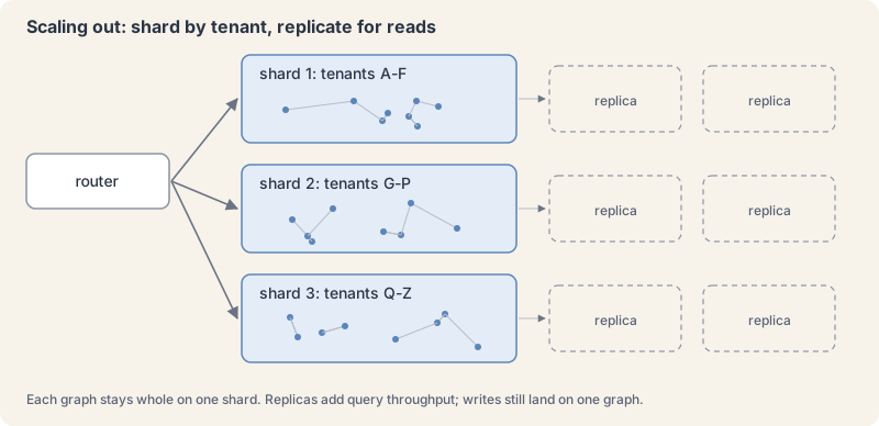
When a single collection outgrows one machine, engines split it into segments or shards, search each one, and merge the partial top-k lists, which costs extra work per query but keeps every graph intact. Tenant-aware sharding avoids that fan-out for most queries. Qdrant’s tiered multitenancy is one built-in version of the idea: small tenants share a shard, and large ones are promoted to their own.

Reads scale with replicas. Writes are the harder problem, because inserting into HNSW mutates the edges of existing nodes, which doesn’t parallelise as neatly as appending to a log. Engines cope by buffering writes and building or merging index segments in the background. The practical advice: batch upserts, spread large backfills over time, and watch index-build lag, not only query latency.

Freshness: accepted is not searchable

Most vector databases acknowledge a write before the new vector is in the index. Until the index catches up, a query may not see it.

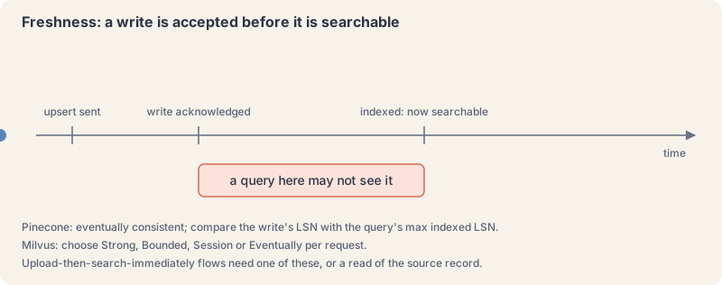
Engines say so, and some give you tools. Pinecone’s freshness guide states that it “is eventually consistent, so there can be a slight delay before new or changed records are visible to queries”. Serverless writes return a log sequence number (LSN), queries report the highest indexed LSN, and when the query’s number is at least the write’s, the write is visible. Milvus lets you choose per request among four consistency levels: Strong, Bounded staleness (the default), Session, which “ensures that all data writes can be immediately perceived in reads during the same session”, and Eventually.

If your product has an “upload a file, then ask about it” flow, you need one of those mechanisms, or a fallback that reads the just-uploaded document directly. Check the specific engine’s guarantee; don’t assume SQL-style read-your-writes.

Memory: quantize, or go to disk

A graph index wants its vectors and edges in RAM, and RAM is the most expensive part of a large deployment. Two escape hatches exist.

Quantization (part 2) shrinks the in-memory copy by 4x (8-bit scalar) up to 32x (binary) or more (product quantization), with the full-precision vectors kept on disk for rescoring a shortlist. For many workloads this is the first and cheapest lever.

Disk-resident indexes go further. DiskANN (Subramanya et al., NeurIPS 2019) showed a graph index (the Vamana graph) that can “index, store, and search a billion point database on a single workstation with just 64GB RAM and an inexpensive SSD”, serving more than 5,000 queries a second with under 3 ms mean latency and 95 percent or better 1-recall@1 on the authors’ benchmark. Compressed vectors stay in memory to guide the search; full vectors and the graph live on SSD. Milvus offers a DiskANN index type, and Elasticsearch’s dense_vector docs list bbq_disk as the default for new float vector fields from 9.4 where the licence allows. Disk-based search costs latency and SSD throughput; treat it as a scale tool, not a default.

Concern	Typical approach
Horizontal scale	Shard by tenant, namespace or collection; don’t split one graph arbitrarily
High write volume	Batch upserts; background segment builds and merges
Freshness	Expect near-real-time; use the engine’s consistency or LSN tools where it matters
Memory pressure	Quantization with rescoring, or a disk-based index

Deletes, updates and re-embedding

Three operations deserve a plan before launch.

• Deletes. As part 2 described, graph indexes usually mark deletions and skip them rather than repairing the graph at once. hnswlib marks elements deleted so they are “omitted from search results” and can reuse the slots later; pgvector cleans up at VACUUM, which “can take a while for HNSW indexes”. Heavy delete traffic degrades a graph over time, and periodic rebuilds are normal.
• Updates. An edited document means new chunks and new vectors, and the old ones must go. Key chunks by document id and version so a re-ingest can replace a document atomically instead of leaving stale chunks behind.
• Re-embedding. A new embedding model means a new space (part 4). Build the new collection alongside the old one, backfill it, evaluate it on your labelled queries, then switch readers over, and keep the old one until you are sure. The embedding bill for a large corpus is real; so is the index build.

Back up the source text and metadata, not only the index. An index can be rebuilt from the chunks; the chunks cannot be rebuilt from the index.

Where a GPU earns its keep

The stage people call “the vector database” is the one that usually needs no GPU. The neural networks around it are where GPU spend pays off, and only if you host them yourself.

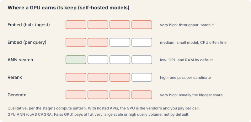
• Hosted APIs for embedding and reranking: you need no GPU of your own. You pay per call for someone else’s; your infrastructure runs the index, which is CPU and memory bound.
• Self-hosted embedding model: a GPU pays for itself once volume is more than trivial, above all for backfills, where large batches keep it busy. Per-query embedding of one short question is light, and a small or quantized model on CPU is often enough.
• Self-hosted reranker: one forward pass per shortlisted candidate on every query, so it bites harder per request. At meaningful query volume a GPU is close to essential; keep the shortlist small and batch all candidates into one call.
• The ANN index: CPU by default. GPU indexes exist and are fast. The Faiss GPU work (Johnson, Douze and Jégou, 2017) made billion-scale GPU search practical, and NVIDIA’s cuVS library ships CAGRA, a GPU graph index whose paper (Ootomo et al.) reports graph construction 2.2 to 27 times faster than HNSW, large-batch query throughput 33 to 77 times higher at 90 to 95 percent recall, and single queries 3.4 to 53 times faster at 95 percent recall, on its benchmarks. Those numbers matter at very large scale or very high query volume, or for building indexes quickly; they are not a reason to put a GPU under a million-vector collection.
• Generation: usually the largest share of end-to-end latency and cost, and usually not your GPU at all if you call a hosted model.

Size GPU budgets around which models you host and how often you call them, never around “we run a vector database”.

Security and compliance

Tenant isolation (part 3) is the first control. A security review will ask about the rest.

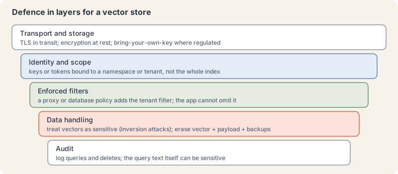
• Encryption in transit and at rest is table stakes for managed services. For regulated data, ask whether you can bring your own key.
• Scoped access. Credentials bound to a namespace, tenant or collection, or a proxy that enforces the scope, so a leaked application key can’t read across tenants.
• Embeddings are not anonymous. Inversion research (Morris et al., 2023) recovered 92 percent of 32-token inputs exactly in its setting. Classify the vector store at the sensitivity of its source data, keep it in the same region, and apply the same retention rules.
• Right to erasure. Under laws such as the GDPR, deleting a person’s data means deleting the vector, the stored chunk text and any copy in backups and derived indexes, not only marking a graph node. With tombstoning indexes, verify that deleted vectors are excluded from results immediately and physically removed on the next rebuild. Per-tenant namespaces or collections (part 3) make whole-customer deletion one operation.
• Audit logging. Log queries and deletes. A query is itself data: the embedded question can be sensitive even when it returns nothing.

Where to go next

The series stops here; these are the topics that build on it, roughly in the order teams run into them:

• Disk-based ANN in depth: how Vamana graphs keep billion-scale indexes on SSD, and what that costs in tail latency. Start with the DiskANN paper and the big-ann-benchmarks competitions.
• Quantization in depth: scalar, product and binary quantization, the recall each gives up, and rescoring strategies.
• Vector database, search engine or Postgres: where pgvector, Elasticsearch and OpenSearch compete with purpose-built engines, and where they don’t.
• Chunking strategies: fixed, structural, semantic and late chunking, and how each interacts with reranking.
• Agent memory: episodic and semantic memory for agents, consolidation, and when retrieval beats a bigger context window.
• Cost modelling: storage, index builds and queries, managed against self-hosted, and how the choice of dimensions drives all three.
• Backup and disaster recovery: snapshotting indexes, cross-region replication, and the real cost of a full re-embed.
• Fine-tuning embedding models: contrastive training on your own relevance data, and when it beats a bigger general model.
• Rerankers compared: cross-encoders, late interaction and language models as judges, on latency, cost and accuracy.

The series, in one paragraph

A vector database finds the nearest points to a query point, approximately and fast, and combines that with filters (part 1). Its index trades recall for speed and memory, and filters and hybrid search change what comes back (part 2). Isolation between tenants is a design decision you enforce below your code (part 3). Quality is set upstream, by the model and the chunking, and known only by measuring recall (part 4). In RAG the database is one box among several, and reranking and graphs fix different failures (part 5). In production it is a stateful, sensitive system like any other, with its own rules for sharding, freshness, hardware and deletion (this part).