Vectors, Plainly, part 1: what a vector database actually does

Part 1 of 6 in Vectors, Plainly, a series on vector databases and retrieval-augmented generation (RAG). One part a day. The series grew out of this site’s own field guide to vector databases, expanded, re-checked against the sources and brought up to date.

A relational database answers one kind of question: which rows exactly match this predicate? A vector database answers a different one: which stored items are closest in meaning to this one? That is not a new storage engine so much as a new query primitive, and most of the confusion around vector databases comes from treating it like the old one.

This first part covers the ground everything else stands on: what an embedding is, what the database adds on top, how “close” is measured, and why the “fields” of a vector are the one part of the schema you never get to design.

Meaning as coordinates

Every item you want to search (a paragraph, a product, an image, a support ticket) is turned into an embedding: a fixed-length list of floating-point numbers produced by a neural network called an embedding model or encoder. Current text models produce lists of a few hundred to a few thousand numbers. OpenAI’s text-embedding-3-small returns 1,536 of them and text-embedding-3-large returns 3,072, according to OpenAI’s launch post; Google’s gemini-embedding-001 and gemini-embedding-2 can return anywhere from 128 to 3,072, per the Gemini API docs.

Each list is a point in a space with that many dimensions. The model was trained so that texts with similar meaning land near each other. “Cheap flights to Tokyo” and “affordable airfare to Japan” share almost no words, yet their points sit close together, because closeness in the space is what the training rewarded.

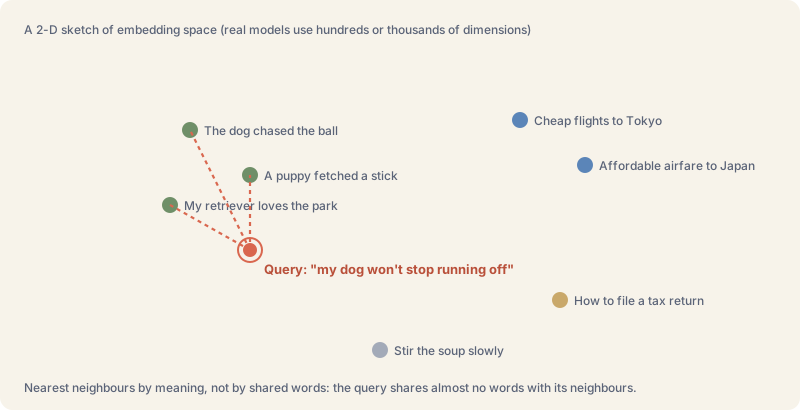
The idea is older than the current boom. The famous illustration is from word vectors: Mikolov, Yih and Zweig (NAACL 2013) showed that the vector for “king” minus “man” plus “woman” lands near “queen”. Sentence-level models followed. Sentence-BERT (Reimers and Gurevych, 2019) made the practical case for embedding whole sentences once and comparing them with cosine similarity: finding the most similar pair among 10,000 sentences took about 65 hours when a BERT model had to read every pair together, and about 5 seconds with embeddings computed once per sentence. That gap is the reason vector search exists as a category.

A diagram like the one above is a two-dimensional cartoon. Real spaces have hundreds of dimensions, and nothing in them lines up with an axis you could label. Keep that in mind; it matters in a moment.

What the database adds

An embedding on its own is just an array. A vector database is three things bolted together:

1. A store for the vectors, plus whatever travels with each one: an id, the original text, and ordinary metadata fields.
2. An index built for approximate nearest-neighbour (ANN) search. Comparing a query against every stored vector is exact but gets slow as the collection grows, so the index trades a little accuracy for a lot of speed. Part 2 opens that box.
3. A query engine that combines similarity with ordinary conditions: tenant_id = "acme", status = "published", price < 50.

Some systems are built for this from the ground up: Pinecone, Qdrant, Weaviate, Milvus, LanceDB, Chroma. Others added vector search to a database that already did something else: PostgreSQL through the pgvector extension, Elasticsearch and OpenSearch through their dense-vector fields, Vespa inside its search and ranking engine. Both families use the same underlying machinery; the differences are in operations, scale, and how well the vector part integrates with everything else you already run.

It helps to see how small the core really is. With pgvector, from the project README:

CREATE EXTENSION vector;

CREATE TABLE chunks (
  id        bigserial PRIMARY KEY,
  tenant_id text NOT NULL,
  body      text NOT NULL,
  embedding vector(1024)
);

-- the five chunks nearest to a query vector, by cosine distance
SELECT id, body
FROM chunks
WHERE tenant_id = 'acme'
ORDER BY embedding <=> $1
LIMIT 5;

<=> is pgvector’s cosine-distance operator. Without an index, that query compares against every row, and the README is explicit that this “provides perfect recall”. Add an approximate index and, in the README’s words, “you will see different results for queries”. That one sentence is the whole bargain of a vector database.

The fields you don’t design

People coming from relational systems ask the same question first: how do I design the fields, and how do I weight them? In a vector database the “fields” are the individual numbers in the vector, and you don’t get to name or design them. Each dimension is a coordinate the embedding model learned during its own training. Dimension 412 does not mean “price” or “colour”; it doesn’t mean anything a person could name, and a different model arranges meaning along entirely different axes.

The “weights” are not per-field knobs either. They are the model’s internal parameters, fixed before you ever call it. What you pass in is text; what comes out is one vector. You never touch an individual dimension.

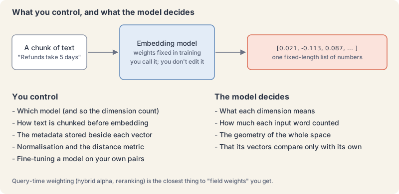
What you do control sits upstream and downstream of the model:

You control	You don’t
Which model you call, and so its dimension count	What any single dimension represents
How text is chunked: a sentence, a paragraph, a page	How much weight the model gave any one word
The metadata stored beside each vector	The geometry of the space
Normalisation and the distance metric	Whether two models’ vectors can be compared (they can’t)
Fine-tuning or training a custom encoder, if you need domain-specific behaviour

Chunking deserves a warning now, because it is the lever people underrate. One vector per page and one vector per sentence make different searches possible: the page vector averages away the detail, the sentence vector loses the context. Part 4 covers how to choose.

The real analogue of “field weights” appears at query time. In hybrid search you blend a vector score with a keyword score, and many engines expose an explicit weight between the two. In reranking, a second model re-scores the top candidates by reading the query and each candidate together. Both come back in parts 2 and 5.

Measuring “close”

Three distance measures cover nearly all practical use:

• Cosine similarity compares the angle between two vectors and ignores their length.
• Dot product combines angle and length.
• Euclidean (L2) distance measures the straight-line gap between the two points.

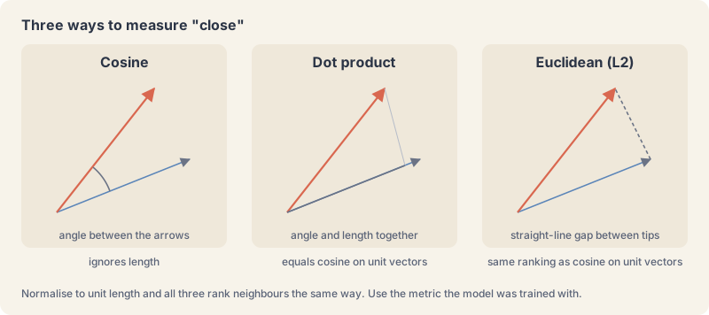
If every vector is normalised to unit length, the three rank neighbours identically: cosine similarity equals the dot product, and Euclidean distance becomes a simple function of it. That is why many pipelines normalise and then use the dot product, the cheapest of the three to compute.

The rule that matters in practice: use the metric the model was trained with, and use the same one at index time and query time. Systems make you declare it. pgvector has separate operators and separate index operator classes for each distance. Elasticsearch’s dense_vector field takes a similarity of l2_norm, dot_product, cosine or max_inner_product, with cosine the default for float vectors. An index built for one metric and queried with another doesn’t fail; it quietly ranks results wrong.

Does the vector keep the text?

No. Embedding is lossy and, for practical purposes, one-way. A chunk of text collapses into a fixed list of floats, and there is no decoder that hands you the original wording back. A vector can tell you what is similar to the source text; it cannot return the source text.

So where does the text in a search result come from? From the record around the vector:

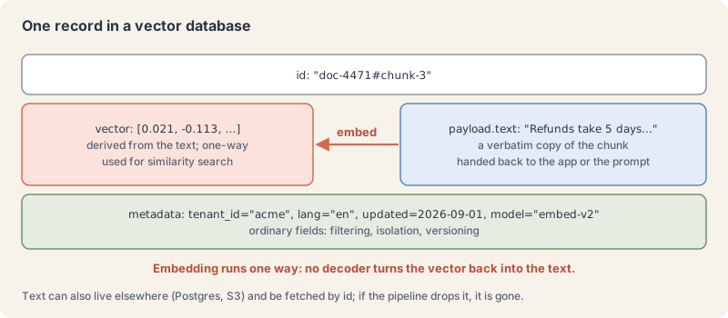
There are three common arrangements:

• Stored as payload beside the vector. The usual pattern. The raw chunk rides in the same record, an exact copy rather than a reconstruction, and the application reads it straight back when the vector matches.
• Stored elsewhere, referenced by id. The vector database holds only vectors and ids; the text lives in Postgres, object storage or a search engine and is fetched in a second lookup.
• Not stored at all. If the ingestion pipeline throws the source away after embedding, it is gone. Nothing in the vector recovers it.

One caveat, and it is a big one. “Not reversible” does not mean “anonymous”. Research on embedding inversion shows that a vector can leak a great deal of its source: Morris et al. (2023) report a method that iteratively corrects and re-embeds text and “is able to recover 92% of 32-token text inputs exactly” in their setting. Treat a vector store as holding the sensitive data it was built from, not a harmless derivative. Part 6 returns to what that means for security reviews.

Do you need one at all?

Not always. A few honest rules of thumb:

• Small collections don’t need an ANN index. An exact scan over tens of thousands of vectors is fast on ordinary hardware, and it is perfectly accurate. Weaviate builds this judgement into its “dynamic” index, which, per its docs, starts as a flat index and switches to HNSW once a collection passes a threshold of 10,000 objects by default.
• If you already run Postgres or Elasticsearch, start there. pgvector or a dense-vector field gives you vectors next to the data they describe, inside transactions and backups you already operate. Move to a dedicated engine when scale, filtering performance or multi-tenancy (part 3) push you there, and not before.
• If users search for exact strings, such as SKUs, error codes and names, pure vector search will disappoint you. You want hybrid search, which part 2 explains.
• If the question is “which rows match”, you want a regular index. Similarity is the wrong tool for exact predicates.

What to carry into part 2

• A vector database finds the nearest points to a query point, usually approximately, and combines that with ordinary filters.
• The model defines the space. You choose the model, the chunking, the metadata and the metric; you never design the dimensions.
• Only vectors from the same model are comparable. Changing models means re-embedding everything.
• The vector doesn’t hold the text, but it can leak it.

---

Next: part 2 of 6, “Inside the index”: how HNSW, IVF and product quantization make nearest-neighbour search fast, and how filtering, hybrid search and reranking shape what comes back. It publishes tomorrow, 29 September.