Vectors, Plainly, part 2: inside the index, from HNSW to hybrid search

Part 2 of 6 in Vectors, Plainly. Part 1 covered embeddings, distance and why you never design the fields.

Comparing a query vector with every stored vector is exact and simple. It is also linear: twice the data, twice the work, on every query. Past a certain size, every vector database stops doing that and builds an approximate nearest-neighbour (ANN) index, which finds most of the true nearest neighbours while looking at a small fraction of the data.

This part opens three index families, the compression tricks that make large indexes fit in memory, and then the query side: filters, hybrid search and reranking, which change results more than most people expect.

Start with no index

Brute force is not a beginner’s mistake. It is exact, needs no tuning and handles deletes trivially. pgvector does it by default, and its README notes that this “provides perfect recall”. For a collection of tens of thousands of vectors, it is often the right answer. Reach for an ANN index when latency or cost says so, and keep a brute-force path around anyway: it is how you measure the index’s recall (part 4).

HNSW: a graph you walk downhill

Hierarchical Navigable Small World graphs, introduced by Malkov and Yashunin, are the dominant ANN index today. Each vector is a node, and edges connect it to some of its near neighbours. The trick is the hierarchy. Every node lives in the bottom layer; a random, shrinking subset also lives in each layer above. The top layers are sparse, so their edges span long distances, like highways. The bottom layer is dense, with short local roads.

A search enters at the top, greedily hops to whichever neighbour is closer to the query, and when no neighbour improves, drops a layer and continues. By the bottom layer it is already in the right neighbourhood and only needs a few short hops.

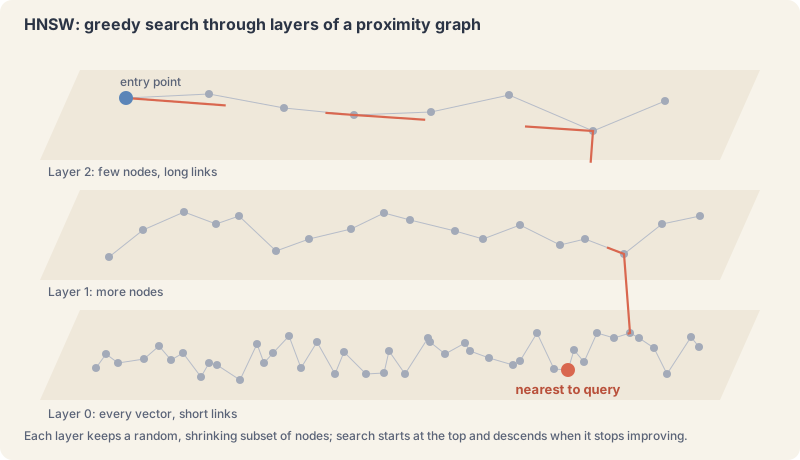
Three parameters matter, and pgvector’s names and defaults are typical:

• m: the maximum connections per node per layer (default 16). More edges, better recall, more memory.
• ef_construction: how many candidates are considered while inserting (default 64). Higher builds a better graph, more slowly.
• ef_search: how many candidates the search keeps in play (default 40, set at query time as hnsw.ef_search). This is your per-query dial between recall and speed.

HNSW’s strengths are excellent recall at low latency and no training step: you can build it on an empty table and insert as you go. Its costs are memory, since the graph’s edges sit beside the vectors and the whole structure wants to be in RAM, and awkward deletes. Removing a node from a graph means repairing the edges that ran through it, so most implementations mark the node deleted and skip it at query time. The hnswlib library’s mark_deleted does exactly that, and later inserts can reuse the slot. pgvector cleans up at VACUUM and warns that this “can take a while for HNSW indexes”. Keep that in mind for part 6, where deletion becomes a compliance question.

IVF: search only the nearest cells

The inverted file index takes the opposite approach. Offline, it runs k-means over the vectors to find a set of centroids (the lists or nlist parameter), and assigns every vector to its nearest centroid’s cell. At query time it finds the few centroids nearest the query (probes or nprobe) and scans only those cells.

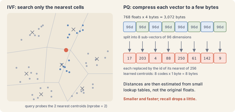
IVF builds faster and uses less memory than HNSW, and the pgvector README says as much, but it gives a worse speed-recall trade-off, and it needs data to train its centroids before it is useful. pgvector’s starting advice is concrete: lists of about rows / 1000 up to a million rows and sqrt(rows) beyond, and probes of about sqrt(lists). A neighbour sitting just across a cell border is the classic miss, which is why nprobe is never 1 in practice.

Product quantization: vectors in a few bytes

A 768-dimension float32 vector takes 3,072 bytes. A billion of them take about 3 TB before any index. Product quantization (PQ), from Jégou, Douze and Schmid (2011), splits each vector into sub-vectors, learns a small codebook of centroids for each slice, and stores only the id of the nearest centroid per slice. With eight slices and 256 centroids each, the vector becomes 8 bytes. Distances are then estimated from small lookup tables instead of the original floats. The paper validated the approach on two billion vectors, and it underpins the IVF-PQ indexes in Faiss, Milvus and LanceDB.

PQ is one member of a family, and modern systems offer several:

• Scalar quantization stores each float as an 8-bit integer: 4x smaller, usually with little recall loss. Qdrant’s docs list it at 4x compression.
• Binary quantization keeps one bit per dimension: up to 32x smaller, and very fast to compare. Qdrant added 1.5-bit and 2-bit variants in v1.15.0 to handle values near zero better.
• Product quantization goes furthest; Qdrant quotes up to 64x, trading more recall and some speed.

The standard way to get the savings without the recall loss is oversampling and rescoring: search the compressed vectors for, say, 2 to 3 times as many candidates as you need, then re-rank that shortlist with the full-precision vectors, which can live on disk. The research is still moving; RaBitQ (Gao and Long, 2024), for example, gives binary-style codes a theoretical error bound.

Defaults are shifting accordingly. Elasticsearch’s dense_vector docs say that since 9.1 a float vector field defaults to bbq_hnsw (HNSW over “better binary quantization”) for 384 or more dimensions, and to int8_hnsw below that. If you upgraded and your memory graph dropped, that is probably why.

The trade-off, in one table

Index	Recall and speed	Memory	Build and updates	Good fit
Brute force (flat)	Exact; slow at scale	Vectors only	Trivial	Small collections, evaluation baselines
HNSW	Best speed-recall balance	High (graph plus vectors)	No training; deletes are awkward	The default for in-memory search
IVF-Flat	Good, tunable with nprobe	Moderate	Needs training data; fast build	Large, fairly static collections
IVF-PQ or quantized HNSW	Lower recall unless rescored	Very low	Needs training (PQ)	Very large collections, memory-bound budgets

There is a fourth family, disk-resident graphs such as DiskANN, which part 6 covers under scaling.

The query side: a query is an embedding

The query path mirrors ingestion. The query text goes through the same model that embedded the data, producing a query vector. The database searches for the top_k nearest stored vectors, and almost always applies a metadata filter at the same time.

Where that filter runs changes what you get back.

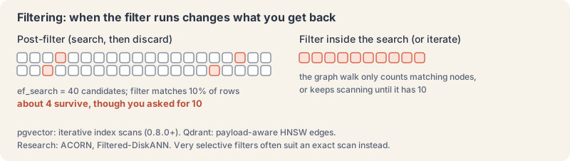
• Post-filtering searches first and discards non-matches. It is simple and it breaks on selective filters. The pgvector README gives the arithmetic: with HNSW’s default ef_search of 40 and a condition matching 10% of rows, “only 4 rows will match on average”. Since 0.8.0, pgvector’s iterative index scans keep scanning until enough rows match.
• Filtering during the search makes the graph walk aware of the filter. Qdrant adds extra graph edges based on indexed payload values so a filtered walk stays connected, and its query planner falls back to a plain scan when the filter is so selective that scanning the matches is cheaper than walking the graph. It also offers ACORN, which looks at neighbours of neighbours when direct neighbours are filtered out.
• Pre-filtering narrows the candidate set first, then searches only that. With a very selective filter, an exact scan of the matches is often both fastest and perfectly accurate.

The research behind this is recent. ACORN (Patel et al., SIGMOD 2024) builds a denser graph so that any predicate leaves a navigable subgraph, and reports “2–1,000× higher throughput at a fixed recall” than prior methods on its benchmarks.

Hybrid search: vectors plus keywords

Dense vectors smooth over exact strings. An order number, an error code, a rare surname or a part number can be nearly invisible to an embedding, while a plain keyword index finds it instantly. Hybrid search runs both a dense vector search and a sparse keyword search (classically BM25) and fuses the two rankings.

The most common fusion is Reciprocal Rank Fusion (RRF) from Cormack, Clarke and Büttcher (SIGIR 2009): each document scores the sum of 1 / (k + rank) over the lists it appears in. The paper fixed k = 60 in a pilot and found the value “near-optimal, but … not critical”, and 60 is still Elasticsearch’s default rank_constant for its RRF retriever.

Here is how that plays out on an illustrative example; the documents are invented, the arithmetic is RRF with k = 60.

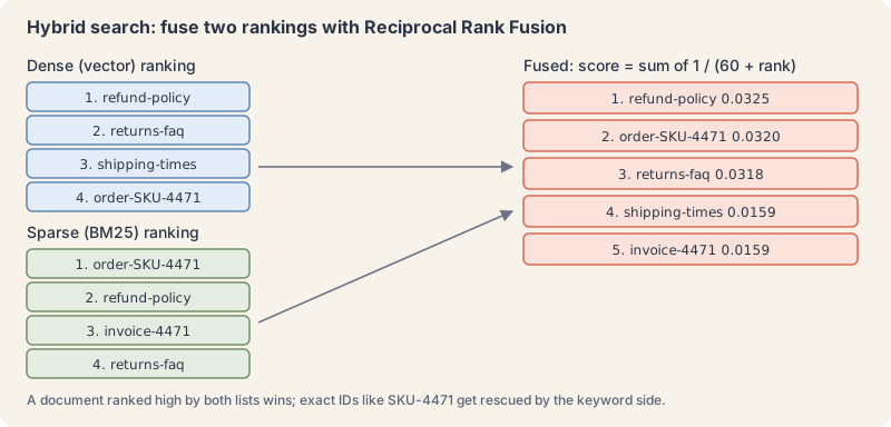
RRF uses only ranks, so it needs no score calibration between two very different scoring systems. The alternative is to normalise the raw scores and blend them with a weight, often called alpha; Weaviate exposes such a weight, and Qdrant offers a distribution-based fusion (DBSF) beside RRF in its hybrid queries. The sparse side need not be BM25: learned sparse models such as SPLADE (Formal et al., 2021) produce weighted keyword vectors, and several engines store them natively.

Hybrid is not an exotic option. The BEIR benchmark (Thakur et al., 2021) found BM25 “a robust baseline” across very different domains, which is a polite way of saying that a dense-only system can lose to 1990s-era keyword scoring when the data doesn’t look like its training set.

Reranking, briefly

The first-pass search compares a query vector with document vectors that were computed separately, which is fast but approximate. A reranker re-scores the shortlist, typically the top 20 to 100, with a heavier model that reads the query and each candidate together. BEIR found that reranking and late-interaction models achieved the best zero-shot results on average, “however, at high computational costs”, which is exactly why they only ever see the shortlist. Part 5 covers how they work and when they pay for themselves.

Tuning without fooling yourself

• Change one knob at a time and measure recall, not just latency: ef_search, nprobe and oversampling each trade one for the other.
• Watch filter selectivity. A query that is fast for a big tenant can return too few results for a small one under post-filtering.
• Budget memory before choosing HNSW for a large collection, and plan quantization with rescoring from the start.
• Add hybrid search as soon as users type identifiers.

---

Next: part 3 of 6, “Multi-tenancy”: how to keep one customer’s vectors out of another’s results, and the namespaces, partitions and filters that organise data inside a vector database. It publishes tomorrow, 30 September.