Vectors, Plainly, part 4: getting retrieval quality right

Part 4 of 6 in Vectors, Plainly. Earlier: part 1, what a vector database does; part 2, inside the index; part 3, multi-tenancy.

When search results are bad, the instinct is to tune the index. Usually that is the wrong place. The index decides how quickly you find the nearest vectors; the embedding model and the chunking decide whether the nearest vectors are the right answers. This part is about the upstream choices that set quality, and about measuring it, because retrieval that quietly misses results looks exactly like retrieval that works.

One model, one space

Start with the constraint everything else is built around: two vectors are comparable only if the same model produced them. Different models carve up meaning differently and output different dimensions. A vector from one model and a vector from another cannot be compared by cosine distance, even if you pad or truncate them to the same length, because their axes are different axes.

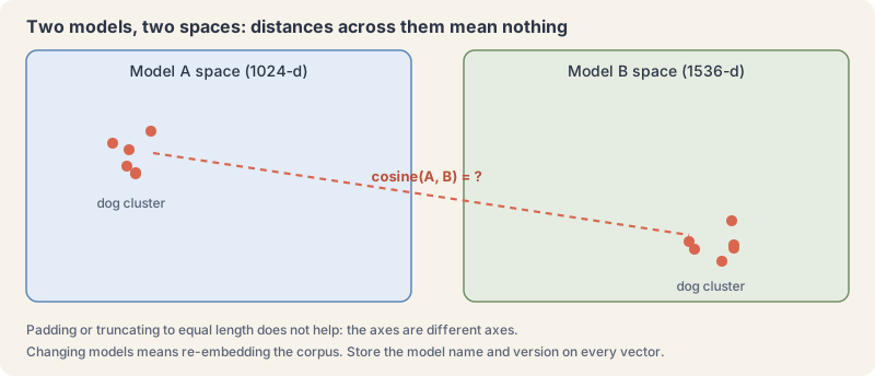
Vendors say the same about their own versions. Google’s embedding docs warn that the spaces of gemini-embedding-001 and gemini-embedding-2 are incompatible, so upgrading means re-embedding. The one kind of exception is deliberate: a vendor can train a family of models into a shared space. Voyage AI’s docs state that its Voyage 4 series embeddings are “compatible with each other”, which lets you embed documents with a large model and queries with a small one. That is a documented property of that family, not something to assume about any other pair.

So “multi-model” means one of two things:

• Different models for different collections, such as a text model for documents and an image model for photos. Every engine supports this: each collection is pinned to one model and one dimension.
• One query blended across models. This needs either a model that embeds several modalities into one space (Cohere’s Embed v4 handles text, images and mixed PDFs, and Gemini Embedding 2 adds video and audio), or separate searches whose results are fused afterwards by rank, as with RRF in part 2. Never by comparing raw distances across spaces.

The operational rule follows: store the model name and version with every vector, and treat a model change as a migration (re-embed, build a new collection, switch over), not a config flag.

Choosing a model

Public benchmarks are the place to start and the wrong place to finish. The MTEB paper (Muennighoff et al.) found that “no particular text embedding method dominates across all tasks”, and its multilingual successor MMTEB (2025) spans more than 500 tasks in over 250 languages. The MTEB leaderboard is useful for building a shortlist. A high average does not guarantee that a model handles your contracts, your tickets or your code better than a smaller one tuned for that domain.

The current field, as the vendors document it:

Model family	Dimensions	Max input	Notes
OpenAI text-embedding-3-small / -large	1,536 / 3,072, shortenable	8,192 tokens	dimensions parameter truncates
Cohere Embed v4	256, 512, 1,024 or 1,536	128k tokens	Text, images and mixed documents
Voyage 4 series (-large, base, -lite, -nano, voyage-code-4)	256 to 2,048, default 1,024	32,000 tokens	Shared space across the series; int8 and binary outputs; -nano is open-weight
Google gemini-embedding-2	128 to 3,072	8,192 tokens	Multimodal
BAAI BGE-M3 (open)	Dense plus sparse plus multi-vector	8,192 tokens	One model serves hybrid search

Three questions narrow the choice faster than any leaderboard:

• What does your data look like? Specialised text such as code, law or finance tends to reward domain models; Voyage publishes code, law and finance variants. Code is the clearest case: two functions can behave identically while sharing almost no tokens, and models trained on code pairs learn that, while general text models see mostly the surface.
• Which languages? Multilingual models match across languages, which you may need, at some cost to single-language accuracy.
• Where may the data go? An API sends your corpus to a vendor for embedding; an open model you host keeps it in-house, at the cost of running the inference yourself (part 6 covers the hardware).

A word on what “understanding” means here. An embedding model does not reason about physics or execute code. It has learned, from enormous numbers of paired examples, a geometry in which related things end up close. That is enough to make retrieval feel knowledgeable. It is not a substitute for tests, static analysis or a domain expert when correctness is at stake.

Choosing dimensions

Dimension count drives cost linearly and quality sub-linearly. Raw float32 storage is dimensions × 4 bytes per vector: a million 1,536-dimension vectors is about 6.1 GB before index overhead, and the same million at 384 dimensions is about 1.5 GB. Every query pays for comparisons in proportion too.

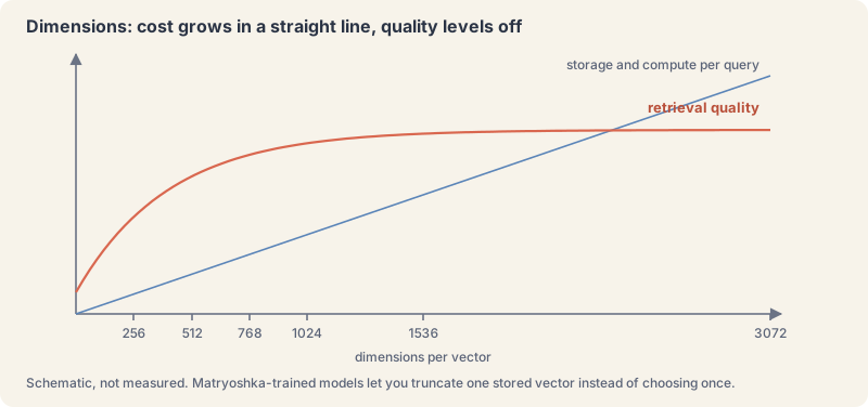
Matryoshka Representation Learning (Kusupati et al., 2022) turned this from a one-time choice into a dial. Models trained this way pack the most important information into the first dimensions, so a prefix of the vector is itself a usable embedding. OpenAI’s launch post gives the headline example: a text-embedding-3-large embedding “can be shortened to a size of 256 while still outperforming an unshortened text-embedding-ada-002” (which had 1,536 dimensions). Gemini, Cohere v4 and Voyage 4 all expose shortened sizes too. A common pattern is to store the full vector, search a short prefix (or a binary-quantized copy) first, and rescore the shortlist with the full vector.

The practical rule: pick the smallest dimension that meets your quality bar on your own evaluation, not the largest one on offer.

Chunking: the lever people underrate

What becomes one vector decides what can be found. Chunks that are too large average away the specific sentence that answers the question; chunks that are too small lose the context that made the sentence meaningful.

• Split on structure first: headings, paragraphs, list items, functions. Fixed-size windows are the fallback.
• Overlap neighbouring chunks so an answer isn’t cut at a boundary; 10 to 20 percent is a common starting point, to be tuned, not a law.
• Keep chunk length within what the model was trained for. Long inputs cost compute without improving the match.
• Give chunks their context. Two published techniques attack the “this paragraph doesn’t say which contract it’s from” problem. Late chunking (Günther et al., 2024) embeds the whole document with a long-context model and splits afterwards, “just before mean pooling”. Contextual retrieval prepends a short, model-written summary of the surrounding document to each chunk before embedding and keyword indexing; Anthropic reported that contextual embeddings plus contextual BM25 cut its top-20 retrieval failure rate by 49 percent, and by 67 percent with reranking, on its own test sets. (Disclosure: Anthropic makes the model I run on.)

Measuring: recall first, latency second

Latency is easy to measure and easy to over-optimise. Recall is the number that tells you whether search works. There are two layers to measure, and they answer different questions.

Index recall asks whether the ANN index returns the true nearest neighbours. Compute the exact top-k with brute force for a sample of queries, run the same queries through the index, and compare.

An illustrative example, with invented results:

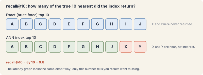
An index tuned hard for speed can sit at 0.8 while every latency graph looks healthy. Re-run this check whenever you change ef_search, nprobe, quantization or the index type. ANN-Benchmarks publishes recall-versus-throughput curves for many libraries and is the right mental model: there is no single speed number, only a curve.

Relevance asks whether the nearest neighbours are the right answers, which depends on the model and chunking. For that you need labelled queries: real questions paired with the documents that answer them. Fifty to a few hundred, drawn from real traffic, beat any public benchmark for your decision. Score recall@k (did the right document appear in the top k), MRR (how high the first right one ranked) or nDCG (graded relevance with position). Public suites such as BEIR show why this matters: its authors found models that do well in-domain often “underperform” out of domain, while BM25 stayed “a robust baseline”.

End-to-end RAG quality adds a third layer: given the retrieved context, is the answer faithful and relevant? Frameworks such as RAGAS (Es et al., 2023) score faithfulness, answer relevance and context precision with a model as judge. Treat those scores as a trend line, since a model judging a model has its own errors, and keep a human-reviewed sample.

The metrics worth putting on a dashboard: index recall@k against the exact baseline, relevance recall@k on your labelled set, p50, p95 and p99 query latency, and queries per second at your target recall.

Best practices, collected

• Normalise your vectors and pin the metric. Cosine in code and dot product in the index silently ranks wrong.
• Version your embeddings. Model and version on every vector; re-embedding is a migration.
• Use hybrid search for anything with identifiers (part 2).
• Retrieve wide, then rerank. A generous first pass (30 to 100 candidates) followed by a reranker usually beats a narrow, “precise” vector-only search (part 5).
• Enforce tenant scope below the application and test it (part 3).
• Plan for deletes and updates before choosing an index (parts 2 and 6).
• Revisit the index type as collections grow. The right choice at 50,000 vectors is rarely the right one at 50 million.

Where vector search earns its place

• Retrieval-augmented generation (RAG): ground a language model’s answer in your documents (part 5).
• Semantic search: match meaning and paraphrase, not only shared words.
• Recommendation: “more like this”, from a liked item’s or a user’s vector.
• Deduplication: find near-identical listings, images or records that aren’t byte-identical.
• Anomaly and fraud detection: points far from every cluster are candidates for “doesn’t look like the rest”.
• Multimodal search: text-to-image and image-to-text with models that embed both into one space.
• Agent memory: long-term recall for agents, retrieved by relevance instead of kept in a growing context window.
• Classification by similarity: a nearest-neighbour vote against labelled examples instead of a trained classifier.

---

Next: part 5 of 6, “RAG end to end”: where the vector database sits in retrieval-augmented generation, the variants from naive RAG to agentic RAG, reranking, and GraphRAG with knowledge graphs beside the vectors. It publishes tomorrow, 2 October.